Tree

Graph

Before diving into tree, let’s understand what is a graph

A graph is a data structure that consists of following two components: - A finite set of vertices also called as nodes. - A finite set of ordered pair of the form (u, v) called as edge. - The pair is ordered because (u, v) is not same as (v, u) in case of directed graph(di-graph). - The pair of form (u, v) indicates that there is an edge from vertex u to vertex v. - The edges may contain weight/value/cost.

Directed Graph

graph LR
  A --> B
  A --> C
  B --> D
  C --> D
  D --> A

Nodes: \{A, B, C, D\}
Edges: \{(A, B), (A, C), (B, D), (C, D), (D, A)\}

Notice that (A, B) is not same as (B, A). That’s because the graph is directed

Undirected Graph

graph LR
  A --- B
  A --- C
  B --- D
  C --- D
  D --- A

In the above graph, (A, B) is same as (B, A). That’s because the graph is undirected

Cycle

A cycle is a path of edges and vertices wherein a vertex is reachable from itself

graph LR
  A --> B
  B --> C
  C --> D
  D --> A

There is a cycle in the above graph. The cycle is \{A, B, C, D\}

graph LR
  A --> B
  B --> C
  C --> D
  C --> A

There is also a cycle in the above graph. The cycle is \{A, B, C\}

Graph Representation

There are two common ways to represent a graph - Adjacency Matrix - Adjacency List

Adjacency Matrix

An adjacency matrix is a square matrix used to represent a finite graph. The elements of the matrix indicate whether pairs of vertices are adjacent or not in the graph.

import networkx as nx
import numpy as np
# graph using adjacency matrix, 4 nodes
graph = [[0, 1, 1, 1], 
            [1, 0, 0, 0],
            [1, 1, 0, 0],
            [1, 0, 0, 1]]


# Create a graph from the adjacency matrix
G = nx.DiGraph(np.array(graph))

# Draw the graph
nx.draw(G, with_labels=True, node_color='lightblue', node_size=500)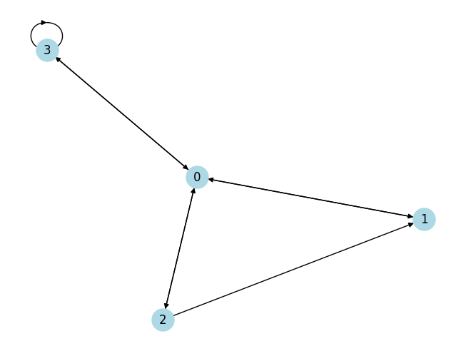

Adjacency List

An adjacency list is a collection of unordered lists used to represent a finite graph. Each list describes the set of neighbors of a vertex in the graph.

The above graph can be represented as follows:

graph = [
    [1, 2, 3],
    [0],
    [0, 1],
    [0, 3]
]

Edge List

Edge list is a collection of unordered pairs used to represent a finite graph. Each pair describes the edge between two vertices in the graph.

graph = [(0, 1), (0, 2), (0, 3), (1, 0), (2, 0), (2, 1), (3, 0), (3, 2)]

Adjacency Matrix vs Adjacency List

Adjacency Matrix	Adjacency List
Takes O(V^2) space	Takes O(V + E) space
Checking if two vertices are connected takes O(1) time	Checking if two vertices are connected takes O(V) time
Iterating over all the edges takes O(V^2) time	Iterating over all the edges takes O(V + E) time

Additional Notes: When the graph is sparse, adjacency list is generally preferred. When the graph is dense, adjacency matrix is generally preferred.

Implicit Graph

An implicit graph is a graph that is not represented by an adjacency list or an adjacency matrix. Instead, the graph is defined by a set of states and transitions between those states.

Example: A chess board is an implicit graph. The states are the positions of the pieces on the board. The transitions are the legal moves that can be made by each piece.

Tree

Tree is a special type of graph where: - There is only one path between any two nodes - There are no cycles

Tree Representation

Adjacency Matrix

Tree can be represented using adjacency matrix. However, it is not a good idea to do so. That’s because adjacency matrix takes O(V^2) space. Since tree is a special type of graph (sparse), it is better to use adjacency list to represent it.

Adjancency List

Tree can be represented as a HashMap, where the key is the node and the value is the list of children.

tree = {}

def add_node(parent, value):
    if parent not in tree:
        tree[parent] = []
    tree[parent].append(value)

add_node(1, 2)
add_node(1, 3)
add_node(1, 4)
add_node(4, 5)
add_node(4, 6)

print(tree)

{1: [2, 3, 4], 4: [5, 6]}

Node Class

We can create a class to represent a node. Each node has a value and a list of children nodes.

class Node:
    children: list["Node"]
    value: int

    def __init__(self, value):
        self.value = value
        self.children = []
    
    def add_child(self, child):
        self.children.append(child)
    
    def __repr__(self):
        return f"Node({self.value}, {self.children})"

root = Node(1)
root.add_child(Node(2))
root.add_child(Node(3))

child = Node(4)
child.add_child(Node(5))
child.add_child(Node(6))

root.add_child(child)

print(root)

Node(1, [Node(2, []), Node(3, []), Node(4, [Node(5, []), Node(6, [])])])

Use Cases

HTML

Well, HTML is a tree. Each node is a tag and the children are the tags inside the tag.

<html>
    <head>
        <title>Tree</title>
    </head>
    <body>
        <h1>Tree</h1>
        <p>Tree is a special type of graph</p>
    </body>
</html>

class Tag:
    name: str
    attributes: dict
    children: list

    def __init__(self, name, attributes=None, children=None):
        self.name = name
        self.attributes = attributes or {}
        self.children = children or []

    def __str__(self) -> str:
        # print in HTML format
        childrens = "".join([str(child) for child in self.children])
        attributes = " ".join([f'{key}="{value}"' for key, value in self.attributes.items()])
        return f"<{self.name} {attributes}>{childrens}</{self.name}>"

tag = Tag("html", children=[
    Tag("head", children=[
        Tag("title", children=[
            Tag("text", children=["Hello, world!"])
        ])
    ]),
    Tag("body", children=[
        Tag("div", attributes={"class": "container"}, children=[
            Tag("h1", children=[
                Tag("text", children=["Hello, world!"])
            ])
        ])
    ])
])

print(str(tag))

<html ><head ><title ><text >Hello, world!</text></title></head><body ><div class="container"><h1 ><text >Hello, world!</text></h1></div></body></html>

Abstract Syntax Tree

Abstract Syntax Tree (AST) is a tree representation of the abstract syntactic structure of source code written in a programming language. Each node is an operator or an operand and the children are the operands of the operator.

That’s the AST for

while b ≠ 0:
    if a > b:
        a := a - b
    else:
        b := b - a
return a

Source: Wikipedia

Binary Search Tree

Binary Search Tree is a tree where each node has at most two children. The left child is smaller than the parent and the right child is greater than the parent.

graph TB
    10 --> 5
    10 --> 15
    5 --> 3
    5 --> 7
    15 --> 13
    15 --> 17

class BST:
    value: int
    left: "BST"
    right: "BST"

    def __init__(self, value):
        self.value = value
        self.left = None
        self.right = None
    
    def insert(self, value):
        if value < self.value:
            if self.left is None:
                self.left = BST(value)
            else:
                self.left.insert(value)
        else:
            if self.right is None:
                self.right = BST(value)
            else:
                self.right.insert(value)
    
    def __str__(self):
        return f"BST({self.value}, {self.left}, {self.right})"

tree = BST(10)
tree.insert(5)
tree.insert(15)
tree.insert(13)
tree.insert(7)
tree.insert(3)
tree.insert(17)

print(tree)

BST(10, BST(5, BST(3, None, None), BST(7, None, None)), BST(15, BST(13, None, None), BST(17, None, None)))

Well, it’s hard to read the above graph. Let’s draw it in a better way. Let’s learn tree traversal.

Tree Traversal

graph TB
    10 --> 5
    10 --> 15
    5 --> 3
    5 --> 7
    15 --> 13
    15 --> 17

Inorder Traversal

Inorder traversal is a type of depth-first traversal. In inorder traversal, we first visit the left subtree, then the root node, and finally the right subtree.

As the name implies, the output of inorder traversal in a BST is sorted.

def inorder(node):
    if node is None:
        return
    yield from inorder(node.left)
    yield node.value
    yield from inorder(node.right)

print(list(inorder(tree)))

[3, 5, 7, 10, 13, 15, 17]

Preorder Traversal

Preorder traversal is a type of depth-first traversal. In preorder traversal, we first visit the root node, then the left subtree, and finally the right subtree.

def preorder(node):
    if node is None:
        return
    yield node.value
    yield from preorder(node.left)
    yield from preorder(node.right)

print(list(preorder(tree)))

[10, 5, 3, 7, 15, 13, 17]

Postorder Traversal

Postorder traversal is a type of depth-first traversal. In postorder traversal, we first visit the left subtree, then the right subtree, and finally the root node.

def postorder(node):
    if node is None:
        return
    yield from postorder(node.left)
    yield from postorder(node.right)
    yield node.value

print(list(postorder(tree)))

[3, 7, 5, 13, 17, 15, 10]

BST

Drawing BST

Having learned tree traversal, we can now draw BST in a better way.

def draw(node, level=0):
    if node is None:
        return
    draw(node.right, level + 1)
    print(" " *  4 * level + str(node.value))
    draw(node.left, level + 1)

draw(tree)

You need to rotate your head to see the tree ;)

Let’s draw in a directory style:

def draw(node, level=0):
    if node is None:
        return
    print("   " * level + "├──" + str(node.value))
    draw(node.left, level + 1)
    draw(node.right, level + 1)

draw(tree)

├──10
   ├──5
      ├──3
      ├──7
   ├──15
      ├──13
      ├──17

Search on BST

The power of BST is that we can search in O(\log n) time. Let’s see how.

tree = BST(10)
tree.insert(5)
tree.insert(15)
tree.insert(13)
tree.insert(7)
tree.insert(3)
tree.insert(17)

draw(tree)

├──10
   ├──5
      ├──3
      ├──7
   ├──15
      ├──13
      ├──17

To search for 7:

Start from the root node 10
Since 7 < 10, go to the left child 5 (we can ignore the whole right subtree -> eliminating half* of the tree)
Since 7 > 5, go to the right child 7
Since 7 = 7, we found it!

The code is pretty simple, remember recursive? :)

\begin{aligned} \text{search}(x, k) &= \begin{cases} \text{False} & \text{if } x = \text{None} \\ \text{True} & \text{if } x.\text{value} = k \\ \text{search}(x.\text{left}, k) & \text{if } k < x.\text{value} \\ \text{search}(x.\text{right}, k) & \text{if } k > x.\text{value} \\ \end{cases} \end{aligned}

def search(node, value):
    if node is None:
        return False
    if node.value == value:
        return True
    if value < node.value:
        return search(node.left, value)
    else:
        return search(node.right, value)
    
print(search(tree, 7))
print(search(tree, 8))

True
False

The problem of BST

BST is a great data structure. It is used in many places. However, it has a problem. The problem is that the height of the tree can be O(n).

It happens when the tree is skewed. For example, if we insert the numbers in ascending order, the tree will be skewed to the right.

tree = BST(10)
for i in range(1, 10):
    tree.insert(i)

draw(tree)

That’s literally a linked list!

Solution

WE NEED TO BALANCE THE TREE!

How? We will learn in the next class :)

Graph

Directed Graph

Undirected Graph

Cycle

Graph Representation

Adjacency Matrix

Adjacency List

Edge List

Adjacency Matrix vs Adjacency List

Implicit Graph

Tree

Tree Representation

Adjacency Matrix

Adjancency List

Node Class

Use Cases

Directory

HTML

Abstract Syntax Tree

Binary Search Tree

Tree Traversal

Inorder Traversal

Preorder Traversal

Postorder Traversal

BST

Drawing BST

Search on BST

The problem of BST

Solution